LAB 11: MODELING OF EPIDEMIC PROPORTIONS AND INITIAL-VALUE ODE PROBLEMS
Mathematics:
Mathematical
modeling of infection diseases among human's population is based on solving the
initial-value problem for a system of ordinary differential equations.
A mathematical model divides a total population into groups of people
interacting to each other with respect to a particular infection disease and
describes the number of people in each group as a function of time. This
project exploits a lethal disease when the total number of population is
divided into four groups: not-yet-infected, infected, medicated and dead
people. The infection is assumed to result from contacts with an infected
individual.
Denote
the time as t, the number of susceptible (not-yet-infected)
people as S = S(t), the number of infected people as I =
I(t), the number of medicated people as M = M(t), and the
number of dead people as D = D(t). The total number of population
is N = S + I + M + D. If the natural birth and death processes
are neglected on the time intervals when the infection disease blows up,
spreads out and eventially disappears, then N is constant in time
t.
Suppose
a is the rate at which the disease spreads per day and also that
the number of people who gets infected is proportional to the number of
interactions between susceptible (S) and infected (I)
people. Then, the rate, at which the number of susceptible people S(t) decreases,
is:
![]() = - a S(t) I(t)
= - a S(t) I(t)
Suppose
r is the death rate of infected people per day and also that the
number of dead people is proportional to the number of infected people (I).
Then, the rate at which the number of dead people D(t) increases,
is:
![]() = r I(t)
= r I(t)
Suppose
b is the constant number of shots per day that save people's
lives and that people who received the medicine can no longer be infected and
are not contageous. Then, the rate, at which the number of medicated people M(t)
increases, is constant as:
![]() = b
= b
Since
the medicine is given only to sick people, it is natural to assume that b
< I(t) for any t > 0. The rate, at which the number
of infected people I(t) changes, can be found from the condition
that the total number of people N remains unchanged for any time t
> 0:
![]() = a S(t) I(t) – r
I(t) – b
= a S(t) I(t) – r
I(t) – b
By
summing all four differential equations above, we confirm that:
![]() =
= ![]() +
+ ![]() +
+ ![]() +
+ ![]() = 0.
= 0.
Objectives:
·
Understand
how to solve the initial-value problems for systems of differential equations
·
Exploit
modeling of the epidemic proportions with the Euler method (discrete
differences)
· Exploit modeling of the epidemic proportions with MATLAB ODE solvers (Runge-Kutta and Adams)
MATLAB script for modeling of the epidemic proportions with the Euler method
In
numerical methods of solving the initial-value problem for systems of
differential equations, the solution is to be found at discrete times: t0,t1,t2,…tn,
starting with the initial time t0 = 0 and
ending at the final time tn = T. If the discrete times
are taken with a constant step size: h = t1 – t0 =
t2 – t1 = … = tn – tn-1,
the derivative of any function f'(tk) at any time t
= tk can be approximated by the first forward divided
difference:
f'(tk) = ![]()
This
is the Euler method for solving the system of differential equations.
Replacing the first derivatives by the first forward differences at the times t
= tk for k = 1,2,…,n; the system of
differential equations becomes the discrete dynamical system, which is suitable
for numerical iterations (loops):
Sk+1
= Sk – h a Sk Ik
Dk+1 = Dk +
h r Ik
Mk+1 = Mk +
h b
Ik+1 = Ik +
h a Sk Ik – h r Ik – h b
Again,
the total number of people is preserved: Nk+1 = Nk.
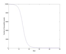
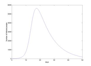
A typical pattern of dynamical behaviour of the number of susceptible (S)
and infected (I) people is shown as a
function of time t:
|
|
|
Steps
in writing the MATLAB script:
- Define N = 10000,
a = 6.90675*10-5, r = 0.1, b = 10.
- Define at time t
= 0, the initial values as I0 = 20, D0
= 0, M0 = 0, and S0 = N – I0.
- Define a final time T
= 50 (days) and the step size h = 0.1 (days). Find
how many iterations n are needed to start at t = 0
and to end at t = T.
- Run a loop in k =
1,2,…,n and find the number of susceptible (S), died
(D), medicated (M) and infected (I) people
at all discrete times t = tk between t
= 0 and t = T. Save vectors t, S, D, M,
and I.
- Plot vectors S,
D, M, and I versus t on four different
graphs.
- Plot the phase plane of
S versus I with the particular solution for 0
 t
t  T.
T.
Exploiting
the MATLAB script:
- Using computations in
the script, find the number of survived people after 15 days.
- Run computations with
no medicine (b = 0) and find the number of survived people
after 15 days.
The
number of survived people at any time t is
R(t) = S(t) + M(t) + I(t) =
N – D(t)
The
number of survived people after 15 days is R = 6673
for b = 0 and R = 8582 for b = 10.
MATLAB script for for modeling of the epidemic proportions with MATLAB ODE solvers
MATLAB
ODE solvers include:
·
ode23:
based on the variable-step Runge-Kutta method of second and third order
·
ode45:
based on the variable-step Runge-Kutta method of fourth and fifth order
·
ode113:
based on the Adams method of the variable order from one to thirteen
·
ode15s:
based on the implicit methods of the variable order for stiff differential
equations
Steps
in writing the MATLAB script:
- Define the system of differential
equations in a separate function M-file "epidem" with two
input arguments: t as scalar and y = [S,D,M,I]
as vector, and with one output argument ydot as
vector-column of the right-hand-sides of the system of differential
equations. Parameters a, b, r can be defined in the body of
the function file.
- Define initial and
final times: t0 and T.
- Define a vector for
initial values: y0 = [S0,D0,M0,I0].
- Call MATLAB ODE
Runge-Kutta solver "ode23" to solve the system of
differential equations.
- Retrive the output of
the ODE solver "ode23" and plot S, D, M, and
I as functions of t.
- Plot the phase plane of
S versus I with the particular solution for 0
< t < T.
Exploiting
the MATLAB script:
- Compare the values for
the number of survivors after T = 15 days with b = 0 and
b = 10 obtained by the Euler method and by the ODE solver "ode23"
- Call other MATLAB
solvers "ode45", "ode113", and "ode15s"
for the same computations.
QUIZ:
- Fill the table of data
values for the number of survivors.
|
|
Euler method |
ode23 |
ode45 |
ode113 |
ode15s |
|
b = 0 |
6673 |
|
|
|
|
|
b = 10 |
8582 |
|
|
|
|
- Compute and plot
functions S, D, M, and I for longer time
interval (T = 100). Explain the behaviour of S, D, M, and
I in terms of the mathematical model of the epidemic
proportions.
- Call MATLAB ODE solver "ode23"
with tolerance control of the absolute global error to be smaller than 10-10.
Find the values for the number of survived people after T = 15
days with b = 0 and b = 10.