CHAPTER 1: INTRODUCTION INTO MATLAB COMPUTING
Lecture 1.5: Plotting
operations and MATLAB graphics
Plotting of functions of one variable:
·
plot: outputs
one vector versus the other vector, the vectors must be of the same structure
and of the same length
% plotting of explicit functions of one variables
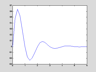
x = 0 : 0.2 : 6; % bad
resolution
y = exp(-x).*sin(pi*x); % y
has the same structure and the length as the vector x
plot(x,y); % the graph is
connected by solid line
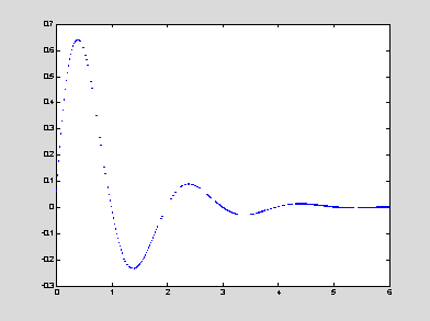
x = 0 : 0.02 : 6; % better
resolution
y = exp(-x).*sin(pi*x);
plot(x,y,'.'); % the graph
consists of data points
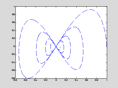
% plotting of
parametric curves (complex numbers)
t = 0 : 0.01 : 8*pi;
z = exp(-0.1*t).*(cos(t) +
i*sin(2*t));
plot(real(z),imag(z),'--'); % the graph is plotted by dashed line
·
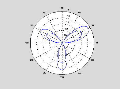
polar: plots a function in polar coordinates (radius versus angle)
y = sin(3*t).*exp(-0.1*t);
polar(t,y); grid on;
·
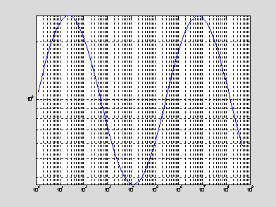
loglog: plots a function in logarithmic coordinates (log(y) versus log(x))
x = exp(2*t);
y = exp(sin(t));
loglog(x,y); grid on;
·
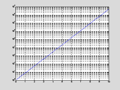
semilogx,semilogy: plots a function in semi-logarithmic coordinates (log(y) versus x or
y versus log(x))
semilogy(t,exp(2*t)); grid on;
·
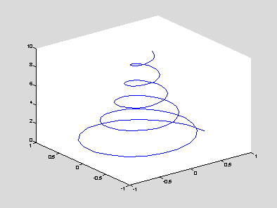
plot3: plots a curve in space of three dimensions
x = exp(-0.2*t).*cos(pi*t);
y = exp(-0.2*t).*sin(pi*t); plot3(x,y,t);
Modifications of plots:
·
data marks (no connection by lines):
o
'.'
– point
o
'+' –
plus
o
'*' –
star
o
'd' –
diamont
o
'o' –
circle
o
'p' –
pentagon
o
's' – square
o
'^'
– triangle
o
'x'
– x-mark
·
line types (no individual points):
o
'-'
– solid line (default)
o
'--' –
dashed line
o
':' –
dotted line
o
'-.' –
dash-dotted line
·
line colors:
o
'r'
– red
o
'y' –
yellow
o
'm' –
magenta
o
'c' –
cyan
o
'g' –
green
o
'b' –
blue
o
'w' –
white
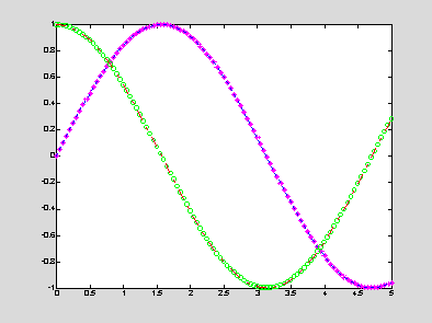
% combination of data marks, line types, and line colors
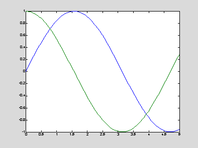
x = 0 : 0.05 : 5;
y = sin(x);
z = cos(x);
plot(x,y,'*m',x,y,':b',x,z,'og',x,z,'-.r');
% check the output and
compare with specification of graphs
plot(x,y,x,z);
% the line types and colors can be automatically selected for each
curve by default
·
fill: draws
filled polygons with a specified color, it can be called instead of "plot"
·
labels and titles:
o
xlabel('x-axis') – the string 'x-axis' is printed as a label for x-coordinate
o
ylabel('y-axis') – the string 'y-axis' is printed as a label for y-coordinate
o
title('The graph of y = f(x)') – the string 'The graph of y = f(x)' is
printed as a title of the plot
o
legend('y = f(x)') – the string 'y = f(x)' is printed in a small sub-window showing
the line type or data marks, used for plotting the function y = f(x)
·
font sizes and line widths:
o
plot(x,y,'—','linewidth',3) – the default line width is 0.5
o
xlabel('x-axis','fontsize',14) – the default font size is 12pt
·
texts:
o
text(x,y,'TextBody') – the string "TextBody" is printed on
the figure, starting at the absolute coordinates (x,y) in pixels
o
num2str, int2str – conversions of a number to string and an integer to string,
respectively
o
LATEX structure of the text:
§
Greek
symbols: \alpha, \beta, \gamma, \epsilon
§
superscripts:
x^2, y^{-2}
§
subscripts:
x_n, y_{i,j}
strText = ['The area of the
circle, A = ',strPi,'*r^2']
% concatenation of three
strings into the text
text(5,10,strText,'fontsize',14,'Color','r');
% setting the properties of the text on a current window
The area of the circle, A = 3.1416*r^2
·
axes and grids
o
axis([x_min,x_max,y_min,y_max]) – set the maximum and minimum values for the
coordinates of the graph (x_min <= x <= x_max; y_min <= y <=
y_max)
§
the
command "axis" must be used after the command "plot"
§
any
line outside the limits will be clipped
o
axis off – the coordinate axes and tic marks are removed (default: axis on)
o
axis square – the figure is reshaped to a square form
o
grid on – a grid is added to the graph (default: grid off)
·
several plots on the same graph:
o
hold on – the command superposes several plots on the same graph, even if another
script is executed (default: hold off)
o
hold off – it is recommended to use this command in the end of the script, if
the command "hold on" has ever been used in the script
When several graphs are plotted,
it is better to define the limits for coordinates in advance. Otherwise, the limits will be the same as
for the first curve. All specifications such as "axis" can be hold
with the command "hold on" before the graphs are plotted on the
figure.
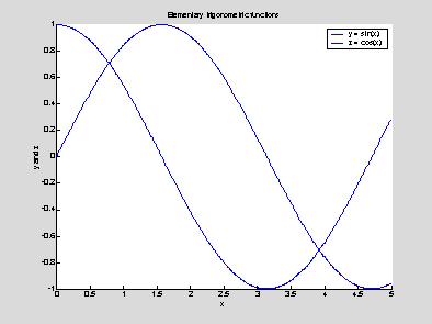
x = 0
: 0.01 : 5; y = sin(x); z = cos(x);
axis([0,5,-1,1]); hold on;
plot(x,y); hold on;
plot(x,z); hold off;
legend('y = sin(x)','z =
cos(x)');
% the number of arguments
correspond to the number of functions plotted
xlabel('x'); ylabel('y
and z'); title('Elementary trigonometric functions');
Operations with figures:
·
figure: opens a new graphic window that is numbered consecutively from the
previous window
·
figure(n): make an existing graphic window (n) the current window; if the
window (n) does not exist, the command opens a new graphic window
numbered by (n) (NB: all graphic commands apply to the current window)
·
pause:
holds up execution of the script and waits for the user to press any key
·
pause(s): holds up execution of the script for s seconds
·
close(n): closes the graphic window (n)
·
close all: closes all graphic windows
·
clf:
clears everything inside the graphic window
·
cla:
clears the plotted curves and redraws the axes
·
figure('Position',[pix,piy,pwx,pwy]): sets the size and shape of the current
window
o
pix,piy – the horizontal and vertical coordinates of the left bottom corner of
the window
o
pwx,pwy – the number of pixels in the width and height of the window
o
default: figure('Position',[232 258 560 420])
·
get(gcf): displays the properties of the current figure, such as size, location,
color map, and many others
·
set(gcf,'PropertyName',PropertyArray): changes the property "PropertyName"
of the current window according to the data in PropertyArray
set(gcf,'DefaultTextColor','blue');
set(gcf,'PaperPosition',[0.25 2.5 4 3]);
·
Property Editor: all properties of the current figure can be edited interactively after
drawing the graphs
·
print:
sends the current figure to the default printer
·
print –dps filename: saves the current figure into a PostScript file
"filename"
·
print –djpeg filename: saves the current figure into a JPEG file "filename"
·
Window Editor: more options for dissemination of research are available interactively
·
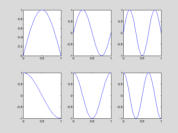
subplot(m,n,k): divide the window into a m by n array of subwindows and places the
current plot into the k-th subwindow (k <= m*n)
subplot(2,3,1), plot(x,sin(pi*x));
subplot(2,3,2), plot(x,sin(2*pi*x));
subplot(2,3,3), plot(x,sin(3*pi*x));
subplot(2,3,4), plot(x,cos(pi*x));
subplot(2,3,5), plot(x,cos(2*pi*x));
subplot(2,3,6), plot(x,cos(3*pi*x));
