CHAPTER 2: MATRIX COMPUTATIONS AND LINEAR ALGEBRA

Lecture 2.5: Plotting of functions of two variables

Functions on rectangular grids:

Consider a function of two variables: z = f(x,y) in the rectangular domain:

D = (x,y): a x b; c y d

Define the discrete interval of the x-axis:

[ a, x₁, x₂, …, x_N, b ]

Define the discrete interval of the y-axis:

[ c, y₁, y₂, …, y_M, d ]

Intersections of vertical lines x = x_n and horizontal lines y = y_m form a rectangular grid of N-by-M interior points and (2*N+2*M) boundary points and 4 corner points. Evaluations of the function z = f(x,y) at the grid points defines an (N+2)-by-(M+2) matrix of values: z_{n,m} = f(x_n,y_m).

· meshgrid(x,y): creates matrices for rectangular grids [X,Y] from vectors [x,y]

x = 0 : 0.5 : 2; % a row-vector of 5 points for the x-axis

y = -3 : 1 : 3; % a row-vector of 7 points for the y-axis

[X,Y] = meshgrid(x,y) % create 5-by-7 matrices for grids of X and Y

% meshgrid is equivalent to: X = ones(7,1)*x; Y = y'*ones(1,5);

X 0 0.5000 1.0000 1.5000 2.0000

0 0.5000 1.0000 1.5000 2.0000

0 0.5000 1.0000 1.5000 2.0000

0 0.5000 1.0000 1.5000 2.0000

0 0.5000 1.0000 1.5000 2.0000

0 0.5000 1.0000 1.5000 2.0000

0 0.5000 1.0000 1.5000 2.0000

Y = -3 -3 -3 -3 -3

-2 -2 -2 -2 -2

-1 -1 -1 -1 -1

0 0 0 0 0

1 1 1 1 1

2 2 2 2 2

3 3 3 3 3

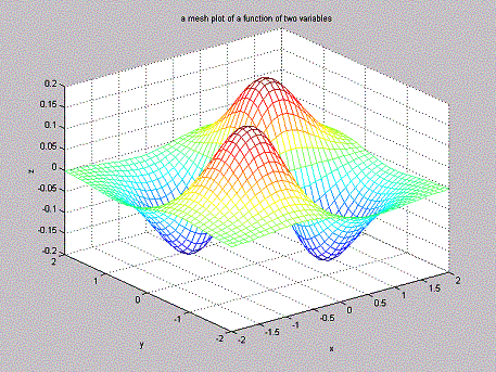
· mesh(x,y,z): plot a shape of function of two variables on a rectangular grid

x = -2 : 0.1 : 2; y = -2 : 0.1 : 2;

% z = x.*y.*exp(-x.^2 – y.^2) : example of a function of two variables

% direct coding of the function z = f(x,y) does not work because x,y,z are row-vectors

[X,Y] = meshgrid(x,y);

Z = X.*Y.*exp(-X.^2-Y.^2);

% pointwise multiplication works now because X and Y are matrices

mesh(X,Y,Z);

title('a mesh plot of a function of two variables');

xlabel('x'); ylabel('y'); zlabel('z');

· contour(x,y,z,label): plots contour lines of a function of two variables on a rectangular grid

• level = L, where L is the number of equally spaced contour levels between the minimum and maximum values of z: z_l = z_min+(z_max-z_min)*(l-1)/(L-1)
• level = V, where V is the vector of contour levels given explicitly
• clabel(h): authomatically annotates the contour levels
• clabel(h,'manual'): allows the user to locate the positions of the labels for contour levels

h = contour(X,Y,Z,10); clabel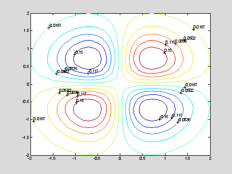(h);

h =

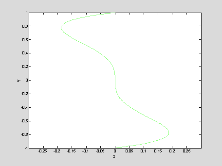
· contour(x,y,z,[0,0]): plots an implicit function of one variable: z = F(x,y) = 0

% y^5 – y^3 = tanh(x) : the implicit function y = y(x) to be plotted

x = -0.3 : 0.01 : 0.3; y = -1 : 0.01 : 1; [X,Y] = meshgrid(x,y);

Z = Y.^5-Y.^3-tanh(X); contour(x,y,Z,[0,0]); xlabel('x'); ylabel('y');

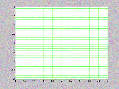
· mesh(x,y,0*y'*x): plots the rectangular grid without any function on the grid

x = 1 : 0.2 : 3; y = -2 : 0.1 : 2;

mesh(x,y,0*y'*x); view([0,0,1]);

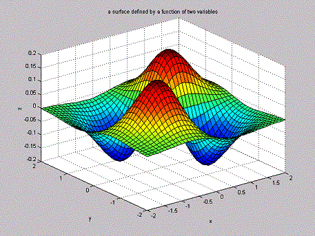
· surf: creates a colorful image of a two-dimensional surface

x = -2 : 0.1 : 2; y = -2 : 0.1 : 2;

[X,Y] = meshgrid(x,y); Z = X.*Y.*exp(-X.^2-Y.^2);

surf(X,Y,Z); title('a surface defined by a function of two variables');

xlabel('x'); ylabel('y'); zlabel('z');

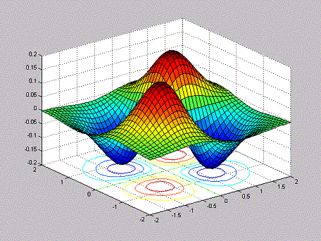
· meshc, surfc: plots contours of the function z = f(x,y) on the (x,y)-plane in addition to the output of functions "mesh" and "surf"

surfc(X,Y,Z)

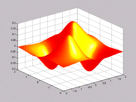
· surfl: creates a two-dimensional surface with lighting

surfl(X,Y,Z); colormap hot; shading interp;

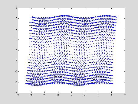
· quiver: plots a two-dimensional vector [u,v] on the plane [x,y], where u = f(x,y); y = g(x,y)

% The system of two differential equations:

% dx/dt = f(x,y) = y; dy/dt = g(x,y) = - sin(x)

% The quiver displays the vector field on the phase plane (x,y)

x = -2*pi:0.25:2*pi; y = -pi:0.25:pi; [X,Y] = meshgrid(x,y);

U = Y; V = -sin(X); quiver(X,Y,U,V,2);

% the last input argument is a scale factor,

% that adjusts the lengths of vectors on the plane

More controls of three-dimensional plots:

· axis([xmin,xmax,ymin,ymax,zmin,zmax]): sets limits of the three-dimensional space

· xlabel, ylabel, zlabel: labels for x, y, z

· view([x,y,z]): changes the view angle of the plot, where [x,y,z] are coordinates of a viewer looking at the origin [0,0,0]

· view([az,el]): changes the view angle of the plot, where az is the azimutal angle in the (x,y) plane, measured from negative y-axis counterclockwise, and el is the elevation angle from the (x,y) plane

• default: view(-37.5,30)

· colormap: changes definition of colors on the color axis

• default: colormap(hsv), where red is assigned to the lowest and highest values of z, while the intermediate values of z are: red, yellow, green, cyan, blue, magenta, red
• each line of "mesh" is painted by the color determined by the average value of the function at the two adjacent points on the line
• each cell of "surf" is painted by the color determined by the average value of the function at the four corner points of the cell
• other colormaps: hot, cold, jet, gray

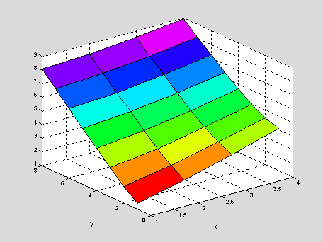
x = 1:4; y = 1:8; [X,Y] = meshgrid(x,y); Z = sqrt(X.^2 + Y.^2);

colormap(hsv); surf(Z); xlabel('x'); ylabel('y');

· shading: changes visualiazation of a surface

• faceted: black border lines and quadrilateral tiles
• flat: no border lines
• interp: no border lines and smooth surfaces

· caxis([zmin,zmax]): specifies the color scheme between the minimal and maximal values of z defined by an user

Remark: it is useful to specify all properties of a figure and keep them with "hold on" before plotting the surface, because plotting operations are time-consuming in space of three dimensions.