CHAPTER 3: NUMERICAL ALGORITHMS WITH MATLAB
Lecture 3.1: Polynomials and
polynomial interpolation
General properties of polynomials:
·
A
general polynomial of order n:
y = Pn(x) = c1
xn + c2 xn-1 + … + cn-1 x2
+ cn x + cn+1
·
Factorization
of polynomials of n-th order by n roots (zeros) x1,x2,…,xn
(possibly, complex or multiple):
y = Pn(x) = c1
(x – x1)*(x – x2)*…*(x – xn)
·
Horner's
method for nested multiplications of polynomials:
y = Pn(x) = ( … (
( ( c1*x + c2 )*x + c3 )*x + c4) … )*x + cn+1
Example:
y = x4 + 2 x3 – 7 x2
– 8 x + 12
y = (x-1)*(x-2)*(x+2)*(x+3)
y = ( ( (x + 2)*x – 7)*x – 8)*x + 12
Polynomials with MATLAB:
·
representation
of polynomials by a row-vector of coefficients
p1 = [ 1,2,-7,-8,12], p2 = [ 2,3,5,9,5]
p2 = 2 3 5 9 5
·
roots: find all zeros of a polynomial from its coefficients
r1 = roots(p1)', r2 = roots(p2)'
r1 = -3.0000 -2.0000
2.0000 1.0000
r2 = 0.2500 - 1.5612i 0.2500 + 1.5612i -1.0000 -1.0000
·
poly: find
coefficients of a polynomial from its zeros
q1 = poly(r1), q2 = poly(r2)
% NB: coefficients q2 are different from coefficients of p2 by a
factor of 2
% The leading-order coefficient c1 is always normalized to 1.
q1 = 1.0000 2.0000
-7.0000 -8.0000 12.0000
q2 = 1.0000 1.5000 2.5000 4.5000 2.5000
%
rounding errors may occur in computations of roots
% Wilkinson's example:
roots(poly(1:20))'
Columns 1 through 11
20.0003 18.9970 18.0118
16.9695 16.0509 14.9319
14.0684 12.9472 12.0345
10.9836 10.0063
Columns 12 through 20
8.9983 8.0003 7.0000 6.0000 5.0000 4.0000 3.0000 2.0000 1.0000
% large
rounding error occurs when highly multiple roots are computed
% y = (x-1)^6
r = [ 1 1 1 1 1 1 ]; p = poly(r), rr = roots(p)'
rr = 1.0042 - 0.0025i 1.0042 + 0.0025i 1.0000 - 0.0049i 1.0000 + 0.0049i 0.9958 - 0.0024i 0.9958 + 0.0024i
·
polyval: evaluate polynomials at a given point
x = [ 0 : 0.2 : 1]; y = polyval(p2,x)
y = 5.0000 7.0272 9.6432 13.1072 17.7552 24.0000
% implementation of the Horner algorithm for nested
multiplication:
function [y] = HornerMultiplication(p,x)
[n,m] = size(x);
y = p(1)*ones(n,m);
for k = 2:length(p)
y = y.*x + p(k);
end
y1 = HornerMultiplication(p1,2.5)
y = HornerMultiplication(p2,x)
18.5625
y =
5.0000 7.0272 9.6432 13.1072 17.7552 24.0000
·
polyder: computes coefficients of the derivative of a given polynomial
% P(x) = c(1) x^n + c(2) x^(n-1) + … + c(n) x + c(n+1)
% P'(x) = n c(1) x^(n-1) + (n-1) c(2) x^(n-2) + … + c(n)
Pder1 = polyder(p1), Pder2 = polyder(p2)
Pder2 = 8 9 10 9
·
polyint: computes coefficients of the
integral of a given polynomial
% P(x) = c(1) x^n + c(2) x^(n-1) + … + c(n) x + c(n+1)
% P'(x) = c(1) x^(n+1)/(n+1) + c(2) x^n/n + … + c(n) x^2/2 +
c(n+1) x + c(n+2)
% c(n+2) are constant of integration (to be defined)
Pint1 = polyint(p1,10) % the constant of integration is 10
Pint2 = polyint(p2) % the constant of integration is 0 (default)
Pint1 = 0.2000 0.5000
-2.3333 -4.0000 12.0000
10.0000
Pint2 = 0.4000 0.7500 1.6667 4.5000 5.0000 0
·
conv: computes
a product of two polynomials
% Let p1 be polynomial of order n, p2 be polynomial of order m,
% conv(p1,p2) is polynomial of order (n+m)
p = conv(p1,p2)
p = 2 7 -3 -18 -12 -57 -47 68 60
·
deconv: computes a division of two polynomials
% Let p1 be polynomial of order n, p2 be polynomial of order m,
% [pq,pr] = deconv(p1,p2) computes the quotient polynomial pq of
order (n-m)
% and the remainder polynomial pr of order (m-1) such that p1 =
p2*pq + pr
[pq,pr] = deconv(p1,p2)
pr = 0 0.5000 -9.5000 -12.5000 9.5000
·
residue: computes partial-fraction
expansion (residues)
% Let p1 be polynomial of order n and p2 be polynomial of order m
% [C,X,R] = residue(p1,p2)
finds coefficients C of the residue terms,
% locations of poles X and
the remainder term of a partial fraction expansion
% of the ratio of two
polynomials p1(x)/p2(x).
% Example: no multiple roots,
% p1(x) C(1) C(2) C(n)
% ---- =
-------- + -------- + ... + -------- + R(x)
% p2(x) x - X(1) x - X(2) x - X(n)
[C,X,R] = residue(p2,p1)
1.2500
4.9500
-2.0000
X = -3.0000
-2.0000
2.0000
1.0000
R = 2
% from partial fraction expansion to the ratio of two polynomials
[q1,q2] = residue(C,X,R)
q1 = 2.0000 3.0000
5.0000 9.0000 5.0000
q2 = 1.0000 2.0000 -7.0000 -8.0000 12.0000
·
polyfit: computes
coefficients of interpolating polynomials of order n that passes through a set of (n+1) data
points
x = [ 1,2,-2,-3,0]; y = [0,0,0,0,12];
p = polyfit(x,y,4) % 4 is the order of the polynomial through 5
data points
pp = poly([1,2,-2,-3]) % the same operation if roots of polynomial are known
p = 1.0000 2.0000
-7.0000 -8.0000 12.0000
pp = 1 2 -7 -8 12
Polynomial interpolation:
Problem: Given a set of (n+1) data points:
(x1,y1);
(x2,y2); …; (xn,yn); (xn+1,yn+1)
Find
a polynomial of degree n, y = Pn(x), that passes through all (n+1) data points.
Assume that the set x1,x2,…,xn,xn+1
is ordered in ascendental order, i.e. x1<x2<…<xn<xn+1.
The polynomial y = Pn(x) is called the
interpolating polynomial for x1<x<xn+1 and
extrapolating polynomial for x < x1 and x
> xn+1.
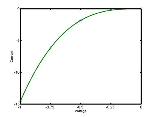
Example: Given a set of five data points for a
voltage-current characteristic of a zener diode
|
Voltage |
-1.00 |
-0.75 |
-0.50 |
-0.25 |
-0.00 |
|
Current |
-14.58 |
-6.15 |
-1.82 |
-0.23 |
0.00 |
The
five points are connected by a polynomial y = P4(x) of
order 4. The data points are shown by blue stars, the polynomial
is shown by green solid line:
Methods:
·
Power
series (Vandermonde interpolation)
·
Lagrange
interpolation polynomials
·
Newton
forward difference interpolation
·
Newton
backward difference interpolation
Vandermonde interpolation:
The (n+1) coefficients ck
of the interpolating polynomial y = Pn(x) are
to be matched with (n+1) data points:
Pn(xk)
= yk.
The
matching conditions produce a system of
(n+1) linear equations for (n+1) unknown
coefficients of the interpolating polynomial:
c1 (xk)n
+ c2 (xk)n-1
+ … + cn-1 (xk)2 + cn xk
+ cn+1 = yk
The
linear system can be solved with the use of MATLAB linear algebra solver.
x = [ -1,-0.75,-0.5,-0.25,-0];
A = vander(x)
y = [
-14.58;-6.15;-1.82;-0.23;-0.00]; c = A\y; c'
xInt = -1 : 0.01 : 0; yInt
= HornerMultiplication(c,xInt);
plot(xInt,yInt,'g',x,y,'b*');
1.0000 -1.0000
1.0000 -1.0000 1.0000
0.3164 -0.4219
0.5625 -0.7500 1.0000
0.0625 -0.1250
0.2500 -0.5000 1.0000
0.0039 -0.0156
0.0625 -0.2500 1.0000
0 0 0 0 1.0000
ans =
0.2133 15.0400
0.3067 0.0600 0

The
Vandermond matrices are ill-conditioned for large n and the
linear algerba solvers produce inaccurate numerical results. Lagrange and
Newton's interpolations are direct methods of finding the interpolating
polynomials, without the necessity to solve linear systems of equations.
Lagrange interpolation:
Lagrange polynomials are defined in the
factorization form:
Ln,j(x) = ![]()
![]()
·
Ln,j(x) is a polynomial of order n
·
Ln,j(xi) = 0 for any i ![]() j
j
·
Ln,j(xj) = 1
The interpolating polynomial y = Pn(x)
has a simple form in terms of the Lagrange polynomials Ln,j(x):
Pn(x) = ![]() = y1Ln,1(x) + … +yn+1Ln,n+1(x)
= y1Ln,1(x) + … +yn+1Ln,n+1(x)
The
interpolating polynomial y = Pn(x) has order n and
it passes through all (n+1) data points. It can be proved that
interpolating polynomials are unique, i.e. the polynomials y = Pn(x)
obtained by the Vandermonde method and by the Lagrange method are the
same polynomials.
function [yi] = LagrangeInter(x,y,xi)
% Lagrange interpolation
algorithm
% x,y - row-vectors of
(n+1) data values (x,y)
% xi - a row-vector of
values of x, where the polynomial y = Pn(x) is evaluated
% yi - a row-vector of
values of y, evaluated with y = Pn(x)
n = length(x) - 1; % order of interpolation polynomial y = Pn(x)
ni = length(xi); % number of points where the interpolation is to
be evaluated
L = ones(ni,n+1); % the matrix for Lagrange interpolating
polynomials L_(n,j)(x)
% L has
(n+1) columns for each point j = 1,2,...,n+1
% L has
ni rows for each point of xi
for j = 1 : (n+1)
for i = 1 : (n+1)
if (i ~= j)
L(:,j) = L(:,j).*(xi' -
x(i))/(x(j)-x(i));
end
end
end
yi = y*L';
Example of Lagrange
interpolation:
x = [ -1,-0.75,-0.5,-0.25,-0];
y = [ -14.58,-6.15,-1.82,-0.23,-0.00];
xInt = -1 : 0.01 : 0;
yInt = LagrangeInter(x,y,xInt);
plot(xInt,yInt,'g',x,y,'b*');