CHAPTER 3: NUMERICAL ALGORITHMS WITH MATLAB

Lecture 3.4: Trigonometric interpolation

General properties of trigonometric series:

Any function y = f(x) that is continuous and periodic function of x with period L can be replaced by the trigonometric (Fourier) series (infinite sum of cosines and sines):

f(x) = a₀ + a_j cos(2jx/L) + b_j sin(2jx/L), 0 x L

where (a_j,b_j) are Fourier coefficients computed from the function f(x) by means of integrals:

a_j = f(x) cos(2jx/L) dx, j = 0,1,2,…,

and

b_j = f(x) sin(2jx/L) dx, j = 1,2,…,

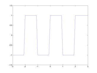
Example: f(x) = sign(x), -1 < x < 1 ; f(x + 2) = f(x), L = 2.

Trigonometric series for sign-function: f(x) = sin(2k - 1) x

Trigonometric interpolation:

Problem: Given a set of (n+1) data points:

(x₁,y₁); (x₂,y₂); …; (x_n,y_n); (x_n+1,y_n+1) ,

such that the values of x are equally spaced on the interval x [0,L] and the values of y are periodic with period of L, i.e. y_n+1 = y₁. Find a finite sum of cosines and sines y = f(x) that connects all (n+1) data points.

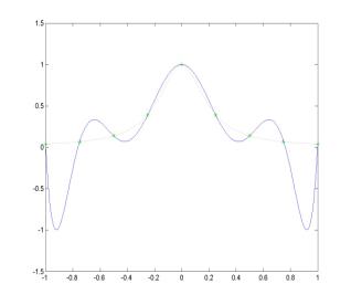
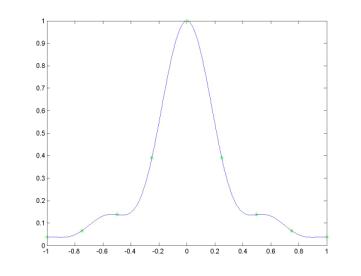
Example: Consider interpolation of the Runge function y = 1/(1 + 25 x²). The polynomial interpolation (on the left) does not produce any good approximation of the Runge function because of the polynomial wiggle. The trigonometric interpolation (on the right) reproduces the Runge function on the interval -1 < x < 1 with sufficiently small error.

Methods:

· Linear systems for Fourier coefficients

· Summation formulas for Fourier coefficients

· Discrete Fourier Tranform

Linear systems for Fourier coefficients:

The interval x [0,L] has the equally-spaced partition at the values of x:

x_i = (i-1)L/n, i=1,2,…,n

The trigonometric interpolation y = f(x) should have n coefficients [a_j,b_j], which are to be found from n equations: y_i = f(x_i). If n is even, i.e. n = 2m, the trigonometric interpolant y = f(x) takes the form:

f(x) = a₀ + a_j cos(2jx/L) + b_j sin(2jx/L) + a_m cos(2mx/L)

The Fourier coefficients are to be found from the linear system:

y_i = a₀ + a_j cos(2 j x_i / L) + b_j sin(2 j x_i / L) + a_m cos(2mx_i/L)

x = -1 : 0.1 : 1; % equally-spaced partition of the interval: –1 < x < 1

y = 1./(1 + 25*x.^2); % values of the Runge function

n = length(x)-1; m = n/2; L = 2;

xx = [x(m+1:n),x(1:m)]'; yy = [y(m+1:n),y(1:m)]';

% continuation of data to the positive interval for x in [0,L]

A = 0.5*ones(n,1); % building the coefficient matrix for linear system

for j = 1 : (m-1)

A = [ A, cos(2*pi*j*xx/L), sin(2*pi*j*xx/L) ];

end

A = [ A, cos(2*pi*m*xx/L) ];

c = A\yy; % computations of Fourier coefficients in a special order

a = [ c(1); c(2:2:n) ]; b = [0; c(3:2:n)]; % coefficients are column vectors

a',b', xInt = -1: 0.01 : 1; % interpolation partition on the same interval

yInt = 0.5*a(1)*ones(1,length(xInt));

for j = 1 : (m-1)

yInt = yInt + a(1+j)*cos(2*pi*j*xInt/L) + b(1+j)*sin(2*pi*j*xInt/L);

end

yInt = yInt + a(m+1)*cos(2*pi*m*xInt/L);

plot(x,y,'*g',xInt,yInt,'b');

ans = 0.5492 0.3442 0.1756 0.0970 0.0499 0.0279 0.0140 0.0084 0.0041 0.0032 0.0010

ans = 1.0e-016 *

0.1228 0.1459 0.0789 0.0692 0.0106 -0.3902 0.1272 0.1426 0.0627

Summation formulas for Fourier coefficients:

When the partition of the interval x [0,L] is equally spaced, the Fourier coefficients [a_j,b_j] can be computed from direct summation formulas:

a_j = y_i cos(2jx_i /L), j = 0,1,2,…,m

and

b_j = y_i sin(2jx_i / L), j = 1,2,…,m-1

These formulas represent the discrete Fourier transform defined at the given set of data points (x_i,y_i).

P = A'*A; % summation formulas follows from the fact that A'*A is diagonal

P(1:6,1:6)

% the discrete cosines and sines are orthogonal with respect to sums!

ans =

5.0000 0.0000 -0.0000 0.0000 -0.0000 0.0000

0.0000 10.0000 -0.0000 0.0000 0 -0.0000

-0.0000 -0.0000 10.0000 -0.0000 -0.0000 0.0000

0.0000 0.0000 -0.0000 10.0000 0.0000 0.0000

-0.0000 0 -0.0000 0.0000 10.0000 -0.0000

0.0000 -0.0000 0.0000 0.0000 -0.0000 10.0000

x = -1 : 0.1 : 1; y = 1./(1 + 25*x.^2);

n = length(x)-1; m = n/2; L = 2;

xx = [x(m+1:n),x(1:m)]'; yy = [y(m+1:n),y(1:m)]';

for j = 0 : m

a(j+1) = 2*yy'*cos(2*pi*j*xx/L)/n;

b(j+1) = 2*yy'*sin(2*pi*j*xx/L)/n;

% inner (dot) product is used for computations

% b(1) = b(m+1) = 0

end

a',b', xInt = -1: 0.01 : 1;

yInt = 0.5*a(1)*ones(1,length(xInt));

for j = 1 : (m-1)

yInt = yInt + a(1+j)*cos(2*pi*j*xInt/L) + b(1+j)*sin(2*pi*j*xInt/L);

end

yInt = yInt + a(m+1)*cos(2*pi*m*xInt/L);

plot(x,y,'*g',xInt,yInt,'b');

ans = 0.5492 0.3442 0.1756 0.0970 0.0499 0.0279 0.0140 0.0084 0.0041 0.0032 0.0020

ans = 1.0e-016 *

0 -0.0833 -0.2220 0 0.1110 0 0.1110 -0.1110 0.0555 -0.0278 0.0471

Discrete Fourier Transform:

The trigonometric sum can be rewritten as a complex Fourier sum:

f(x) = c_j exp( 2i*), i = , 0 x L (1)

where c_j = n (a_j - ib_j) / 2 and c_-j = n (a_j + ib_j ) / 2. The complex Fourier coefficients c_j are found from the summation formulas:

c_j = y_k exp(-2i*), j = 0,,…, (2)

Given data points (x_k,y_k) for k = 1,…,n and n = 2m, formulas (2) are usually referred to as the discrete Fourier transform (DFT), while formulas (1) at the points (x_k,y_k) are referred to as the inverse discrete Fourier transform (IDFT). We use a simple observation:

c_-j = exp(2i*) = exp(2i*) = exp(2i*) = c_n-j

Then, the discrete and inverse discrete Fourier transforms can be regrouped for positive indices:

c_j = y_k exp(-2i*), j = 0,1,2,…,n-1

and

y_k = c_j exp( 2i*).

These formulas are valid only at the discrete data points (x_k,y_k). In order to actually interpolate the function y = f(x) beyond the data points (x_k,y_k), we would need to use the formula for trigonometric interpolation with:

a_j = Re(c_j); b_j = -Im(c_j); j = 0,1,…,m,

where m = n/2.

· fft: computes the discrete Fourier transform

· ifft: computes the inverse discrete Fourier transform

x = -1 : 0.5 : 1; y = 1./(1 + 25*x.^2); % data points

n = length(x)-1; m = n/2; L = 2;

xx = [x(m+1:n),x(1:m)]'; yy = [y(m+1:n),y(1:m)], yy = yy';

for j = 0 : m

a(j+1) = 2*yy'*cos(2*pi*j*xx/L)/n;

b(j+1) = 2*yy'*sin(2*pi*j*xx/L)/n;

end

a =a, b =b % Fourier coefficients of trigonometric series

c = fft(yy); c = c'

aF = 2*real(c(1:m+1))/n; bF = -2*imag(c(1:m+1))/n;

aF = aF, bF = bF % Fourier coefficients derived from FFT

yF = ifft(c) % the same function y is recovered, i.e. yF = ifft(fft(y)) = y

yy = 1.0000 0.1379 0.0385 0.1379

a = 0.6572 0.4808 0.3813

b = 1.0e-017 *

0 0 0.4710

c = 1.3143 0.9615 0.7626 0.9615

aF = 0.6572 0.4808 0.3813

bF = 0 0 0

yF = 1.0000 0.1379 0.0385 0.1379

In order to compute the function y = f(x) at data points different from (x_k,y_k), the trigonometric sum should be used:

f(x) = a₀ + a_j cos(2jx/L) + b_j sin(2jx/L) + a_m cos(2mx/L)

Trigonometric approximation:

If m < n/2, the trigonometric sum only approximates the function y = f(x) in the least-square sense, since there are more data points (x_k,y_k) than the Fourier coefficients (a_j,b_j) to be found.

· fft(y,N), ifft(y,N): compute the trigonometric interpolation if N = length(y), the trigonometric approximation if N < length(y) and the trigonometric interpolation with padded zeros for y if N > length(y)

x = 0 : 0.01 : 1; y = x.*(1-x); % data points

n = length(x)-1; m = n/2; L = 1;

xx = x(1:n)'; yy = y(1:n)';

N = 10; mN = N/2; c = fft(yy,N);

a = 2*real(c(1:mN+1))/N; b = -2*imag(c(1:mN+1))/N;

aa = a', bb = b'

xInt = 0: 0.01 : 1; yInt = 0.5*a(1)*ones(1,length(xInt));

for j = 1 : (mN-1)

yInt = yInt + a(1+j)*cos(2*pi*j*xInt/L) + b(1+j)*sin(2*pi*j*xInt/L);

end

yInt = yInt + a(mN+1)*cos(2*pi*mN*xInt/L);

plot(x,y,'*g',xInt,yInt,'b');

aa = 0.0843 -0.0100 -0.0093 -0.0092 -0.0091 -0.0091

bb = 0 -0.0277 -0.0124 -0.0065 -0.0029 0

The trigonometric approximation with N = 10 is shown on the left.

The trigonometric interpolation with N = n = 100 is shown on the right.