Numerical integration is much more reliable process compared to numerical differentiation. The round-off error in computing the sum of values Ik, where k = 0,1,...,n, is always constant which does not depend on the rule of numerical integration. This constant is bounded by the product of the integration interval T and the maximal round-off error er in computer's representation of numbers. Thus, if the truncation error of the numerical integration rule can be reduced by a recursive algorithm (see Lecture 3.5), the resulting numerical approximation represents the exact value of the integral accurately subject to a constant total round-off error.
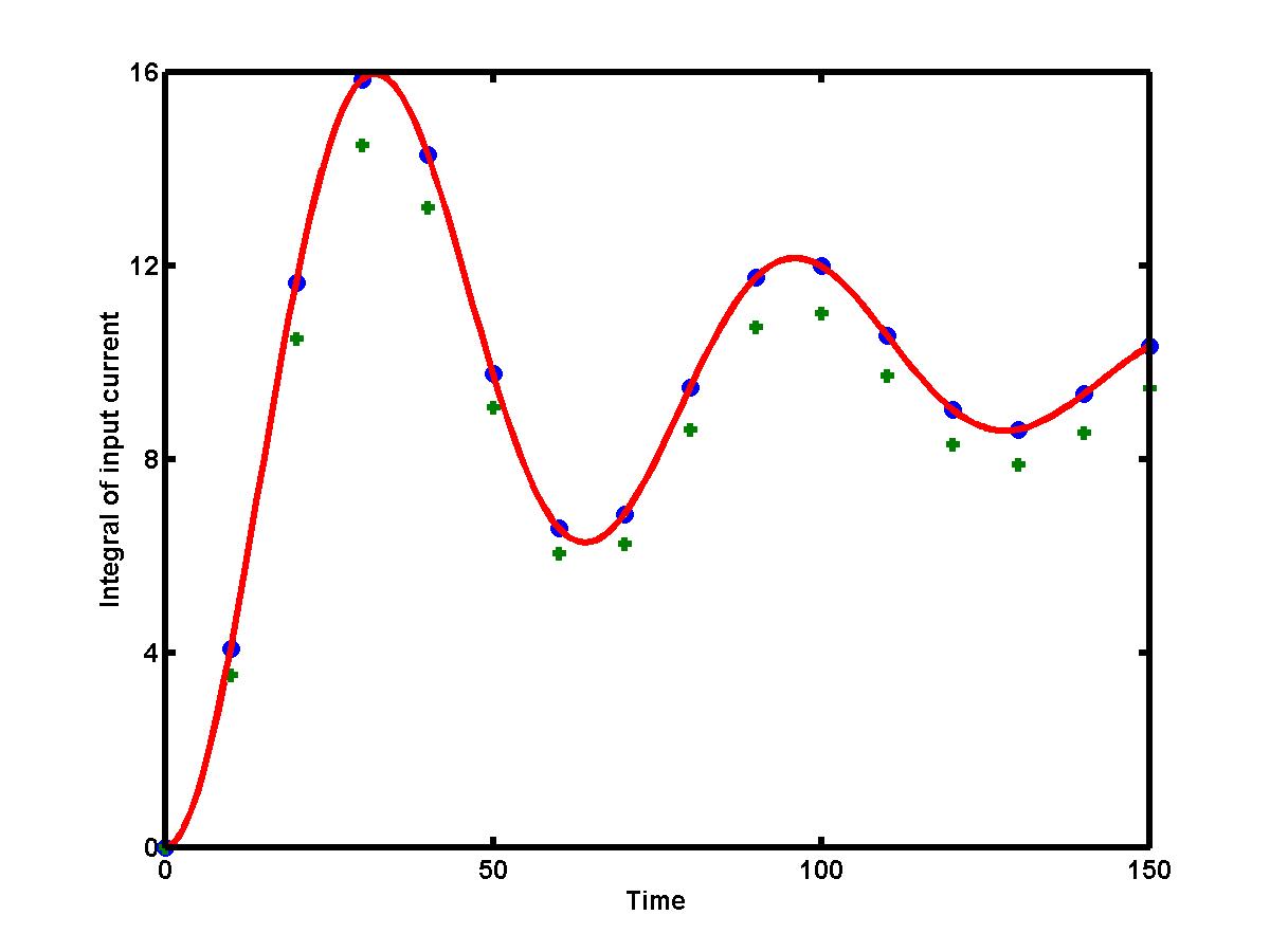
The truncation error can be reduced by two different ways: by reducing the step size h and by using the higher-order integration formula of the order of O(h2), O(h4), and so on. If the step size h between two adjacent values Ik becomes smaller, the truncation error of the numerical integration rule decays. For example, if the step size is reduced by half, the global truncation error of the composite trapezoidal rule is reduced by four. The figure below presents the results from the use of two composite trapezoidal rules on the current I = I(t) (view the data values for the current). The approximations are obtained with step size h = 10 (green pluses) and with step size h = 5 (blue dots), versus the exact integral ST[I(t)] (red solid curve). The error of the composite trapezoidal rule clearly reduces with smaller step size h (blue dots are closer to the exact red curve compared to the green pluses).
The figure also shows that the truncation error for the integral grows with the length of the interval. It is the global truncation error of numerical integration over the interval t = 0 and t = T. The global truncation error is distinguished from the local truncation error, the latter error occurs when the integral between two adjacent points is replaced by a trapezoid.
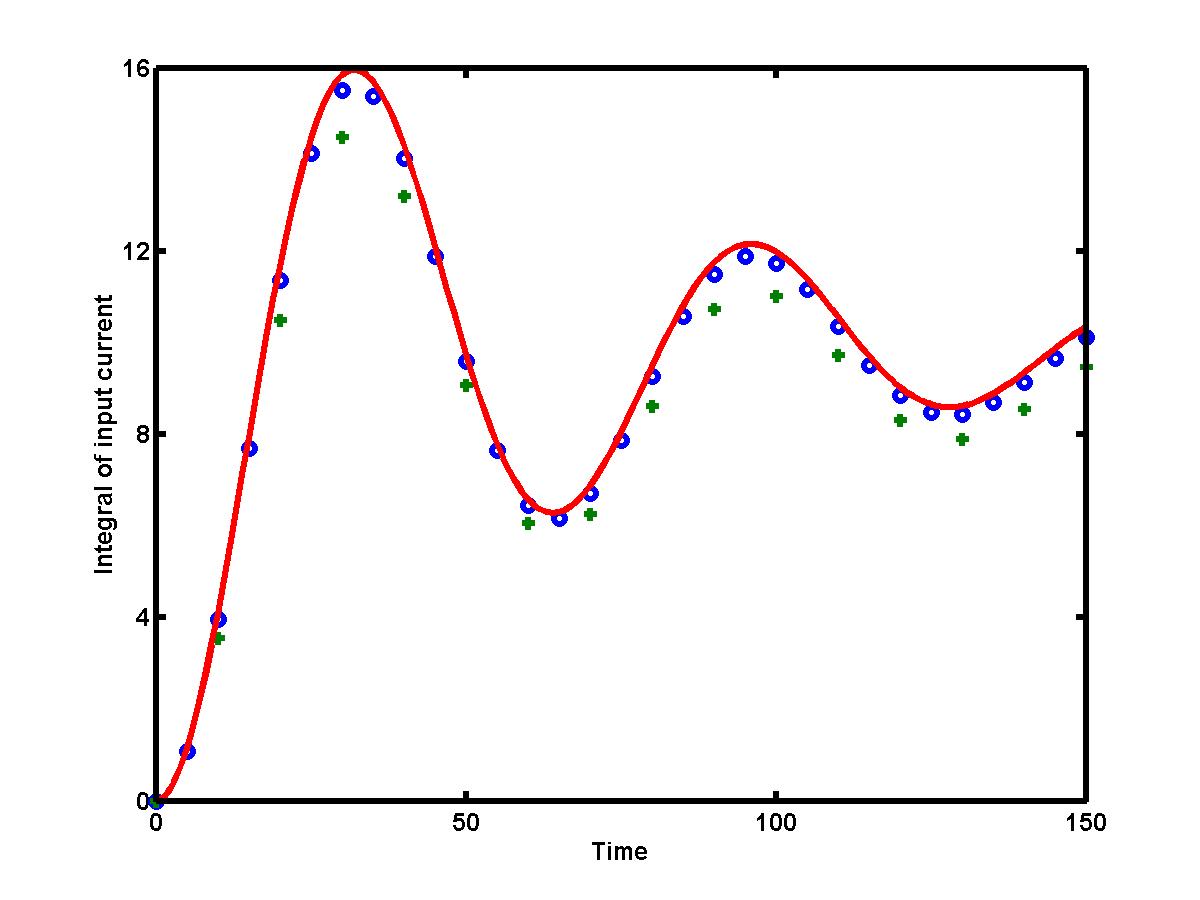
In many cases, the data samples are given with a fixed step size h that can not be controled. If this is the case, the numerical approximation for the integral can be improved by using a higher-order integration rule, such as the Simpson's rule. Romberg integration algorithm (see Lecture 3.5) allows to construct a sequence of higher-order integration rules starting with few computations of the composite trapezoidal rule. The figure below presents comparison of the composite trapezoidal rule (green pluses) and the composite Simpson's rule (blue dots) for the integral of the current I = I(t). The step size h is the same for both the numerical integrations: h = 10. The exact integral ST[I(t)] is shown by red solid curve. The composite Simpson's rule is clearly much more accurate than the composite trapezoidal rule.