Lecture 2.3:
Linear and cubic splines

Higher-order polynomial interpolation is rarely used for practical purposes because of a polynomial wiggle, i.e. high swings of the interpolating polynomials between the data points. Instead, most of computational algorithms use the idea of splines, i.e. piecewise interpolation. The MATLAB functions interp1(x,y,xi,'linear') and interp1(x,y,xi,'spline') are also based on piecewise linear and cubic interpolation.

Linear splines

The linear spline represents a set of line segments between the two adjacent data points (V_k,I_k) and (V_k+1,I_k+1). The equations for each line segment can be immediately found in a simple form:

I_k(V) = I_k + ( I_k+1 - I_k) ( V - V_k ) / (V_k+1 - V_k),

where V = [V_k,V_k+1] and k = 0,1,...,(n-1). When the linear spline is applied to the voltage-current data for a zener diode, the interpolating algorithm produces the following picture:

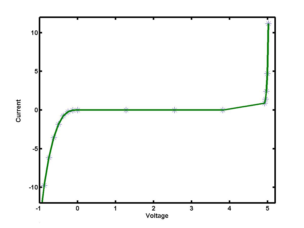
The resulting curve is clearly not smooth, with sharp corners at the data points. However, the piecewise interpolation represents the "exact" curve I = I(V) better that the Lagrange or Newton polynomial interpolation. The linear spline is constructed for each interval V = [V_k,V_k+1] independently and it matches the data values (V_k,I_k) for k=0,1,...,n.

Cubic splines

We can improve the appearance of the piecewise interpolation by matching not only the data values but also the slopes and the concavities of each individual interpolating segment at the interior data points. For (n+1) data values (V_k,I_k) we would have n conditions to match the values I(V_k), (n-1) conditions to match the slopes I'(V_k) and (n-1) conditions to match the concavities I''(V_k), i.e. 3n - 2 conditions (equations). Cubic splines would be good candidates for such interpolation:

I_k(V) = I_k + a_k ( V - V_k ) + b_k ( V - V_k )² + c_k ( V - V_k )³,

where V = [V_k,V_k+1] and k = 0,1,...,(n-1). Indeed, the cubic splines have 3n unknown coefficients (more than required). Two more conditions should be added separately at the ends of the interpolating interval, i.e. at the points V = V₀ and V = V_n. These end-point or boundary conditions are set due to additional assumptions on appearance of the interpolating curve. The simplest conditions follow from the assumption that the concavity is zero at the ends. This is a definition of a natural cubic spline.

A suitable computational algorithm to define the coefficients of cubic splines solves a WELL-posed linear system for concavities I''(V_k) = m_k subject to the boundary conditions: m₀ = m _n = 0 (for natural splines). Provided the solution for m_k is found for k = 1,2,...,(n-1), the coefficients of the cubic splines are

a_k = ( I_k+1 - I_k ) / (V_k+1 - V_k ) - (2 m_k + m_k+1) ( V_k+1 - V_k ) / 6
b_k = 0.5 m_k, c_k = 1/6 ( m_k+1 - m_k ) / (V_k+1-V_k)

Note that the cubic spline reduces to the linear spline if concavities are neglected, i.e. all m_k are zeros. When the cubic spline is applied to the voltage-current data for a zener diode, the interpolating algorithm produces the following picture acceptable both for further work and visualization:

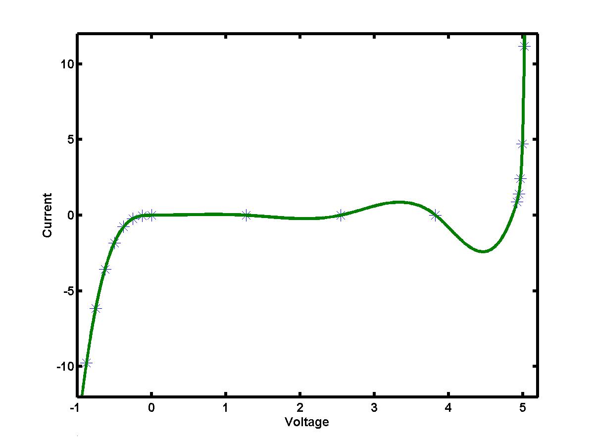
The error of the cubic spline interpolation is O(h⁴), where h is the maximum spacing between the data points.