LAB 8: MARKET WEEKLY REPORTS AND CUBIC SPLINE INTERPOLATION

Mathematics:

Interpolation problems are problems of finding a curve that passes through specified points in the plane. Fitting a curve through points in the plane encounters commonly in analyzing experimental data, in ascertaining the relations among variables and in design work. This project exploits ideas of piecewise cubic spline interpolation for a presentation of market weekly data in the form of a smooth "well-behaved" curve. For the week of February 11-15, 2002, the market indices were registered at the closing bells as follow:

Toronto Stock Exchange 300:

Day of Week	Monday	Tuesday	Wednesday	Thursday	Friday
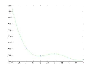
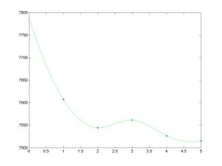
Index Value	7607.40	7544.60	7561.20	7526.40	7515.30

Nasdaq Index:

Day of Week	Monday	Tuesday	Wednesday	Thursday	Friday
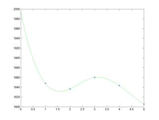
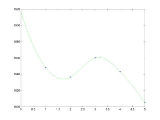
Index Value	1848.20	1836.50	1860.20	1843.40	1805.20

With the use of cubic splines, the data can be represented by a smooth curve as seen in the weekend news reports:

Suppose a set of (n+1) data points is given in the (x,y) plane:

(x₁,y₁); (x₂,y₂); …; (x_n,y_n); (x_n+1,y_n+1)

In our case, n = 4. Also the points are equally spaced in the x-direction, such that the distance between the x-coordinates (step size) is:

h = x₂ -x₁ = x₃ -x₂ = … = x_n+1 -x_n

Let y = S(x) denote a smooth interpolating curves that connects the given data points. The cubic spline interpolant y = S(x) consists of cubic polynomials y = S_j(x) that connect two consecutive data points: (x_j,y_j) and (x_j+1,y_j+1):

y = S_j(x) = a_j + b_j (x - x_j ) +c_j (x – x_j)² + d_j (x – x_j)³, x_j < x < x_j+1

Coefficients (a_j,b_j,c_j,d_j) are found from the conditions that piecewise cubic spline interpolants y = S_j(x) form a continuous curve with continuous first and second derivatives at all points. Both the slopes and the curvatures of the interpolants y = S_j(x) are matched continuously, so that the resulting interpolating curve y = S(x) shows up as a smooth curve in viewer's eyes. Eyes of a viewer cannot distinguish any sudden changes in third and higher derivatives of the curve y = S(x).

Denote m_j = S_j''(x_j) for j = 1,2,…,n,n+1. The coefficients (a_j,b_j,c_j,d_j) of the cubic spline interpolants y = S_j(x) are found from the values of m_j as:

a_j = y_j , b_j = - h, c_j = , and d_j =

The values of m_j are found from a system of (n-1) equations:

m_j-1 + 4 m_j + m_j+1 = ( y_j-1 – 2 y_j + y_j+1 ), j = 2,…,n

The linear system is under-determined, since two values of m_j are still unknown and two more equations have to be added to the system of (n-1) equations. There are several ways to specify the two additional conditions required to obtain a unique cubic spline through the points: (i) natural spline, (ii) parabolic runout spline, and (iii) cubic runout spline.

Objectives:

· understand the algorithm for setting cubic spline interpolants with different end-point conditions

· exploit the cubic spline interpolation and achieve the best visualization of the market weekly reports

MATLAB script for natural cubic spline interpolation:

The natural cubic spline interpolation is prescribed by the end-point conditions:

m₁ = 0; m_n+1 = 0

The natural spline conditions are equivalent to the conditions that the second derivative of the cubic spline y = S(x) is zero at the end points. Thus, the natural spline approaches to the end points x = x₁ and x = x_n+1 as a straight line. The natural spline tends to flatten the interpolating curve at the end points, which may be undesirable:

The linear system for values of m_j (j = 2,…,n) for natural spline interpolation is set in the matrix form: A m = b, where

A = , m = , b =

Steps in writing the MATLAB script:

1. Assign the given data values to vectors x for weekdays, y for TSE300 index, and z for NASDAQ index.
2. Initialize and compute the coefficient matrix A and the vector of right-hand-sides b for each data set.
3. Compute the values of m_j for j = 1,2,…,n,n+1 for each data set.
4. Compute coefficients (a_j,b_j,c_j,d_j) of the cubic spline interpolants y = S_j(x).
5. For two data sets, plot the cubic spline interpolants for a small-sized partition x_int between [0,5], where 0 stands for Monday opening bell and 5 stands for Friday closing bell.
6. Plot points of the corresponding data sets at the same graphs.

Exploiting the MATLAB script:

Compute the values of the cubic spline interpolant in middle of Wednesday.

Answer: In the middle of Wednesday: TSE 300 = 7551.66; NASDAQ = 1848.57

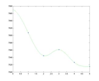
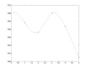
MATLAB script for parabolic runout spline interpolation:

The parabolic runout spline interpolation is prescribed by the end-point conditions:

m₁ = m₂; m_n+1 = m_n

The parabolic runout spline conditions are equivalent to the conditions that the spline y = S(x) reduces to a parabolic curve on the first and last intervals. Thus, the parabolic runout spline approaches to the end points x = x₁ and x = x_n+1 as a parabolic curve. The parabolic runout spline is neither flat nor curved at the end points, i.e. it may be a reasonable compromise for a better visualization of the interpolating curve:

The linear system for values of m_j (j = 2,…,n) for parabolic runout spline interpolation is set in the matrix form: A m = b, where

A = , m = , b =

Steps in writing the MATLAB script:

1. Assign the given data values to vectors x for weekdays, y for TSE300 index, and z for NASDAQ index.
2. Initialize and compute the coefficient matrix A and the vector of right-hand-sides b for each data set.
3. Compute the values of m_j for j = 1,2,…,n,n+1 for each data set.
4. Compute coefficients (a_j,b_j,c_j,d_j) of the cubic spline interpolants y = S_j(x).
5. For two data sets, plot the cubic spline interpolants for a small-sized partition x_int between [0,5], where 0 stands for Monday opening bell and 5 stands for Friday closing bell.
6. Plot points of the corresponding data sets at the same graphs.

Exploiting the MATLAB script:

Compute the values of the cubic spline interpolant in middle of Wednesday.

Answer: In the middle of Wednesday: TSE 300 = 7552.95; NASDAQ = 1849.30

QUIZ: "MATLAB script for cubic runout spline interpolation:

The cubic runout spline interpolation is prescribed by the end-point conditions:

m₁ = 2*m₂ -m₃; m_n+1 = 2*m_n -m_n-1

The cubic runout spline conditions are equivalent to the conditions that the spline y = S(x) reduces to a single cubic curve on the first two and last two intervals. Thus, the values of m₁ and m_n+1 are extrapolated from inside conditions that the first two cubic spline interpolants y = S₁(x),y = S₂(x) and the last two cubic spline interpolants y = S_n-1(x),y = S_n(x) coincide identically. The cubic runout spline produces a curve with pronounced curvature at the end points, which may be undesirable. The linear system for values of m_j (j = 2,…,n) for cubic runout spline interpolation is set in the matrix form: A m = b, where

A = , m = , b =

Steps in writing the MATLAB script:

1. Assign the given data values to vectors x for weekdays, y for TSE300 index, and z for NASDAQ index.
2. Initialize and compute the coefficient matrix A and the vector of right-hand-sides b for each data set.
3. Compute the values of m_j for j = 1,2,…,n,n+1 for each data set.
4. Compute coefficients (a_j,b_j,c_j,d_j) of the cubic spline interpolants y = S_j(x).
5. For two data sets, plot the cubic spline interpolants for a small-sized partition x_int between [0,5], where 0 stands for Monday opening bell and 5 stands for Friday closing bell.
6. Plot points of the data sets at the same graphs.

Exploiting the MATLAB script:

1. Compute the values of the cubic spline interpolant in middle of Wednesday.
2. Use MATLAB function "spline" to compute the values of the spline interpolant in middle of Wednesday.
3. Compute the norm of the difference between the cubic spline interpolants produced by MATLAB function "spline" and by the cubic runout spline. Show that the MATLAB function "spline" uses in fact the cubic runout spline conditions.