![]() If the data set is corrupted by measurement noise, i.e. the data values are
rounded roughly, the numerical interpolation would produce a very stiff
curve with sharp corners and large interpolation error. Another technique
is used instead: it is based on numerical approximation of given data values.
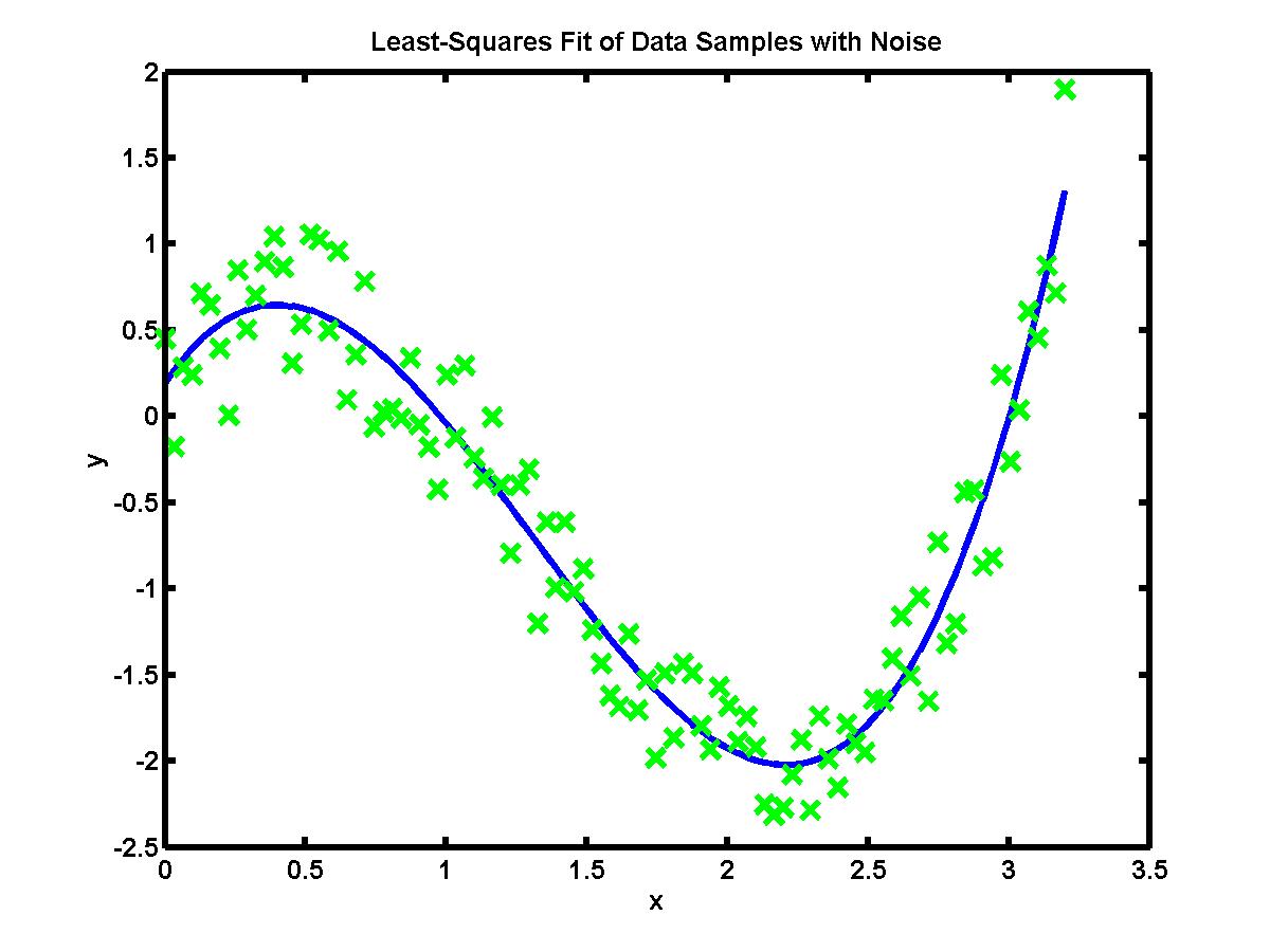
The figure below shows numerical approximation of more than hundred of
data values by a cubic polynomial (click the image to enlarge):
If the data set is corrupted by measurement noise, i.e. the data values are
rounded roughly, the numerical interpolation would produce a very stiff
curve with sharp corners and large interpolation error. Another technique
is used instead: it is based on numerical approximation of given data values.
The figure below shows numerical approximation of more than hundred of
data values by a cubic polynomial (click the image to enlarge):

Numerical approximation works when the data values reproduce a simple characteristic, e.g. a polynomial of lower order or an exponential function. Such characteristics are usually obtained as solutions of theoretical models (differential equations). Therefore, the methods of numerical approximation give a tool to compare theoretical models and real data samples.
We shall study the least squares numerical approximation. This is the problem to find the best fit function y = f(x) that passes close to the data sample: (x1,y1), (x2,y2), ..., (xn,yn) such that a total square error between the data values and the approximation is minimized, where the total square error is
E = (y1 - f(x1))2 + (y2 - f(x2))2 + ... + (yn - f(xn))2,
The linear least squares fit or linear regression is the linear function y = f(x) = ax + b, where the coefficients a and b are computed from statistical parameters of the data sample:
f(x) = ymean + Sxy (x - xmean) / Sxx,
where xmean is the mean of x-values, ymean is the mean of y-values, Sxx is the variance of x-values, and Sxy is the covariance between x and y values.
The exponential function y = c exp(d x), where c and d are constants, can be equivalently rewritten as a linear function:
log(y) = d x + log(c)
If the data sample is given for (xk,yk), then (i) compute the data for Xk = xk and Yk = log(yk), (ii) find the coefficients a and b of the linear least square fit through the data sample (Xk,Yk), and (iii) compute coefficients c and d as c = exp(b) and d = a (follow for these elementary transformations!).
One can try to match coefficients of the polynomial least squares fit by solving a linear system. The linear system is obtained by minimizing the total square error E. However, the linear system is ill-conditioned for large n (number of data points). As a result, a better method is used in practice. The method consists of two phases: (i) constructing a set of orthogonal polynomials through the given data points (xk,yk) and (ii) computing coefficients of the linear combination of orthogonal polynomials from a well-conditioned linear system.