![]() Suppose you use a zener diode for a voltage regulator circuit (to filter out the
small sinusoidal ripple voltage and to refine the constant power signal).
You need to use the voltage - current characteristic I = I(V) in order to
compute the steady-state voltage drop across the electric network. However,
this function is not amenable to representation with a simple analytical expression.
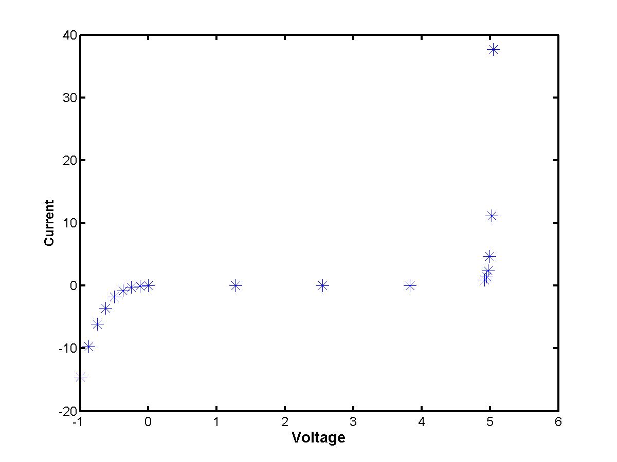
Instead, measurements are available only for several data points. Plotted on a graph
"Voltage vs. Current", they look like this (click the image to enlarge):
Suppose you use a zener diode for a voltage regulator circuit (to filter out the
small sinusoidal ripple voltage and to refine the constant power signal).
You need to use the voltage - current characteristic I = I(V) in order to
compute the steady-state voltage drop across the electric network. However,
this function is not amenable to representation with a simple analytical expression.
Instead, measurements are available only for several data points. Plotted on a graph
"Voltage vs. Current", they look like this (click the image to enlarge):
How to connect the data values and to reproduce a simple analytical representation of the voltage - current characteristic? This is a problem of numerical interpolation: find a function I(V) that passes through each of the data points (Vk,Ik) for k = 0,1,2,...,n (total number of data values is n+1). We shall work only with polynomial interpolation, when the function I = I(V) is thought to be a polynomial. There are two principally different ways to construct the interpolating polynomial. One is to look for an uniform polynomial of a higher degree that passes through all given data points at once (see Lectures 2.1 and 2.2). The other is to construct independent polynomials of lower degree on individual sub-intervals and to match them at the given data points (see Lecture 2.3).
Given (n+1) data points, we shall look for a polynomial of degree n that has (n+1) undefined coefficients:
I(V) = a0 + a1 V + a2 V2 + a3 V3 + ... + + an-1 Vn + an Vn
The (n+1) coefficients must be matched with the (n+1) data values. There are two numerically accurate algorithms to find the same polynomial I(V) based on Lagrange and Newton interpolating polynomials. Both the methods use the following matching conditions:
I(Vk) = Ik, k=0,1,2,...,n,
that give (n+1) linear equations for (n+1) unknown coefficients of the interpolating polynomial. One can think about a straightforward method to solve the resulting linear system. However, the system is numerically ILL-conditioned and produces inaccurate numerical results. Instead of solving the linear problem, we follow to the Lagrange and Newton's methods to define the interpolating polynomials.
Consider the following (Lagrange interpolating) polynomial Ln,k(V) as
(V-V0) (V-V1) ... (V-Vk-1)
(V-Vk+1) ... (V-Vn)
---------------------------------------------------------------
(Vk-V0)
(Vk-V1) ... (Vk-Vk-1)
(Vk-Vk+1) ... (Vk-Vn)
It is clear that the Lagrange interpolating polynomial Ln,k(V)
Based on these three key properties, we verify that the following polynomial
I(V) = I0 Ln,0(V) + I1 Ln,1(V) ... + In Ln,n(V)
has degree n and passes through all (n+1) data points. Between the data points, the Lagrange interpolating polynomial is expected to approximate the unknown "exact" function I = Iexact(V) with the error bound:
| I(V) - Iexact(V) | < C | (V-V0) (V-V1) ... (V-Vn) |,
where C is a constant defined at the interval V = [V0,Vn]. If the data values are equally spaced, i.e. h = Vk - Vk-1 for any k=1,2,...,n, the maximal error is order of O(hn+1) (see Lecture 1.2). Although the error vanishes at any given data point (Vk,Ik), the error between the data values could be large for interpolating polynomials of larger degrees n.
![]()