| Mathematical Modeling | PDE Theory | Spectral Theory | Evolution Equations |
|---|
Spectral analysis is a central method in studies of linear systems with the superposition principle. Fourier spectral representations are used in quantum mechanics, wave propagation, harmonic analysis, and signal processing. If f(x) is a square integrable function on real line, it can be represented in a dual (spectral) space with the integral transforms:
f(x) = (2π)-1 ∫F(k)eikxdk, F(k) = ∫ f(x)e-ikxdx.The Fourier transform F(k) corresponds to a spectral density of the harmonic oscillations eikx between the wavenumbers k and k+dk. The inverse Fourier transform f(x) corresponds to a spectral decomposition of a function f(x) over a continuous linear combination of the harmonic oscillations eikx. If the function f(x) is C1 continuous everywhere in x, the Fourier transform F(k) is C1 continuous everywhere in k, and the Fourier integrals converge.
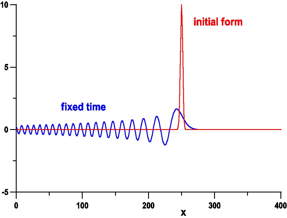
Linear differential equations, especially initial-value problems for wave equations, can be easily solved with the use of spectral decompositions such as the Fourier transforms. For example, small-amplitude long water waves are described by the linear Korteweg--de Vries equation:
ut + uxxx = 0, u(x,0) = f(x).The Fourier transform solves the problem on real line of x in a spectral k space as
u(x,t) = (2 π)-1 ∫ U(k,t) eikxdk, U(k,0) = F(k)Since the Fourier transform F(k) has the property: F'(k) = ik F(k) for a square integrable function f(x), the time evolution of the spectral density U(k,t) is trivial, Ut = i k3 U(k,t), with the straightforward solution: U(k,t) = F(k) exp(ik3t). As a result, the exact solution u(x,t) of the initial-value problem for the linear KdV equation is a spectral superposition with density F(k) of linear waves exp(i(kx - ω(k) t)), where ω(k) = -k3 is the dispersion relation.
Inverse scattering transform generalizes spectral analysis for solution of initial-value problems for nonlinear differential equations. For example, the inverse scattering transform is applied to solve the nonlinear KdV equation:
ut + uxxx - u ux = 0, u(x,0) = f(x).The KdV equation is related to the spectrum of the stationary Schrodinger equation on a real line of x with a t-dependent potential u(x,t):
- w''(x) + u(x,t) w(x) = λ w(x)Quantum theory develops spectral analysis of the stationary Schrodinger equation. If initial data f(x) is a square integrable function on real line, the spectral data consists of the continuous spectrum at λ = k2 > 0 with eigenfunctions w(x;k) and a finite-dimensional discrete spectrum at λ = - p2n < 0 with eigenfunctions wn(x). The spectral decomposition of the potential u(x,t) over eigenfunctions of the continuous and discrete spectrum takes the form:
u(x,t) = (2π)-1 ∫ ρ(k,t) w(x;k) dk + ∑ ρn(t) wn(x),where ρ(k,t) and ρn(t) are coefficients of the spectral decomposition. The time-evolution of the spectral data is trivial with the simple solution:
ρ(k,t) = ρ(k,0) exp(i k3 t), ρn(t) = ρn(0) exp(pn3 t).The initial values for the spectral data have to be found from spectral analysis of the stationary Schrodinger equation with the initial potential u(x,0) = f(x).
|
|

|
Inverse Scattering for Linear Operators with Algebraic Potentials | |
|
|
Exact Solutions of Integrable Reductions of KP Hierarchy |